Algorithms menu. Several categories are in there : Selection, Color, Layout, Measure, Size, General. They modify the properties of the graph elements.
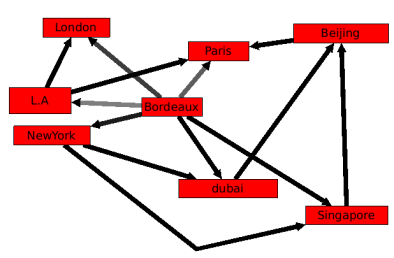
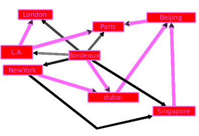
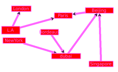
The induced Sub-Graph algorithm can be used to obtain the edges that are between selected nodes.
Here is an example :Before :

After :

The Algorithm of Kruskal is used to create a minimum spanning tree out of a connected graph.
It is divided in several steps :
- Make a list of the edges starting with the "shortest" one, ending with the "longest one".
- Add all edges with their from/to nodes to the tree as long as you don't have any cycle.
This selection algorithm is able to select the loops of a graph. A loop is an edge that has the same source and target.
This selection algorithm highlights the multiple-edges also named parallel-edges in a graph.
Two edges are parallel only if they both have the same target and same source.
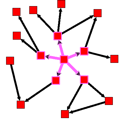
Algorithm documentationDistance: number of edges to follow.Direction: 0 means directed, 1 reverse directed, 2 undirectedStarting nodes: the selected nodes of this selection property ( boolean ) will be used as starting nodes.
Before :
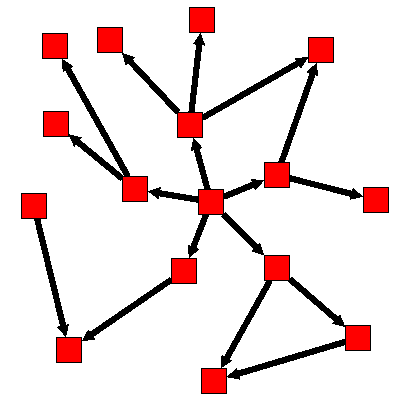
After :
Algorithm documentation
This selection algorithm can be used to select a sub-graph without any cycle.
Algorithm documentationThis algorithm can be used to create a set of spanning trees out of the graph.
A tree is a special kind of graph that has the following properties :Has a root (a starting point node).
A node have severals sons and their is only one edges targeting each sons.
Doesn't have any cycle.
- A leaf is an "ending node".
The metric mapping algorithm can be used to re-color the nodes of the graph after using a measure ( the section called “Measure” ) algorithm.
This Algorithm takes 5 parameters :Property: Property is a metric value. It is used to affect scalar values to graph items.Colormodel: Color can be either 1 or 0. 1 for RGB interpolation and 0 for HSV interpolation.Type:If type is checked, the color mapping will be uniform, which means that if you have 2 nodes with the property value equals to 0, there will be 2 nodes colored in "color1" .
If type is not checked, the color quantification will be linear, which means that if you have 2 nodes with the property value equals to 0, there will be 1 node colored in "color1" and an other with a lighter color1.
Color1: Color1 will be the color of the node that has the lowest value (according to the Property field)Color2: Color2 will be the color of the node that has the highest value (according to the Property field)
Let's take an example :
As you can see here is a graph where no metric values has been computed.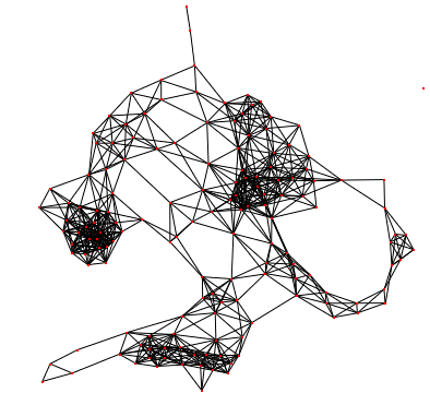
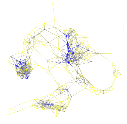
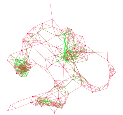
This algorithm can only be used on simple graphs (graphs with no loops).
The cluster algorithm is a measure algorithm that can determine whether or not a graph is a "small-world network". The clustering measure is a local measure that gives the connections rate of a node and its neighbors.
Let's take an example :
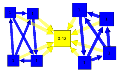
On this graph, and by looking at the clustering measure, you can see 2 "communities" (nodes in blue) and a hub (node in yellow).the hub is the only way to connect the two communities.
For more details, please visit http://en.wikipedia.org/wiki/Clustering_coefficient.
Algorithm documentationType : Is the type of degree you want to compute. In : Edges that comes onto the node. Out : Edges that are going away from the node. InOut : Using both (in and out).
Metric : This parameter can take all double properties, but by default it will take : None, 'viewBorderWidth', 'viewMetric' and 'viewRotation'. If you choose none, the degree of the node will be the sum of the edges. If you choose the 'viewMetric' value, degree of the node will be the sum of edges wiewMetric property. As of viewBorderWidth and viewRotation.
This plug in compute the eccentricity of each node, eccentricity is the maximum distance to go from a node to all others. In this version the value is normalized (1 means that a node is in the center of the network, 0 means that a node is the more eccentric in the network). The eccentricity will be saved in the viewMetric property of each node.
Algorithm documentation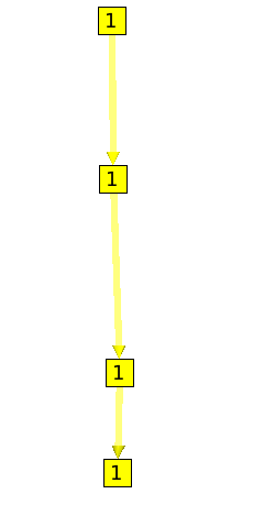
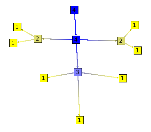
Parameters :
All nodes :If not checked, the algorithm will choose a node (a source node) and will apply the algorithm to this node only. If checked, the algorithm will be applied to all nodes.Type :This parameter can take 3 different values : Register which will force the algorithm to give an indication on the degree of ramification (for trees), Stack, that will force the algorithm to give an indication on the number of nested cycles (for graphs), and at last, All, that will ask the algorithm to use both registers and stack.
For more information please visit http://en.wikipedia.org/wiki/Strahler_Stream_Order
Algorithm documentationGraph must be simple (no loops).
This algorithm will compute the strength of edges. Every edges with small values are important in the way that their removal can disconnect two connected components. Every edges with a high value metric may belong to a strongly connected component.
Algorithm documentation- 1 : Paris, New York, L.A, Madrid.
- 2 : Paris, Berlin.
- 3 : Berlin, Moscow, Prague.
A connected component is a maximal connected subgraph. Two nodes are in the same connected component if and only if there exists a path between them.
After running the algorithm, the index of the connected component of a node is saved in its viewMetric property. It is the same for the edges.
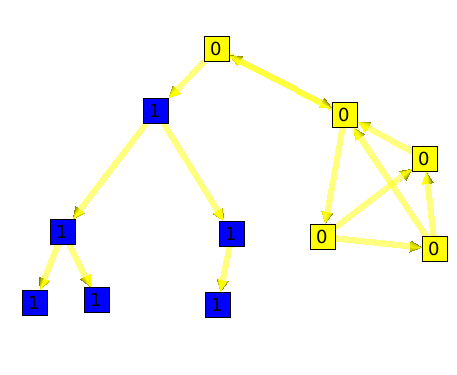
For more details please visit : Wikipedia:Connected ComponentAlgorithm documentationThe connected tree component algorithm can be useful to find parts of a graph that are trees. Here is an example :
Following is a graph with on the left side, a tree. This graph forms a unique connected component.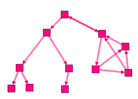
- The Source of e1 is S1 and Target is S2 .
- The Source of e2 is S2 and Target is S1.
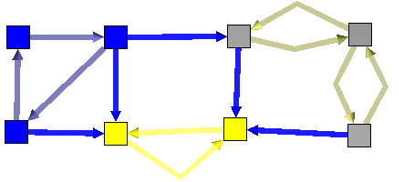
These form a partition of the graph.
Here is an example :Before :
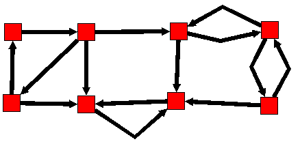
After :

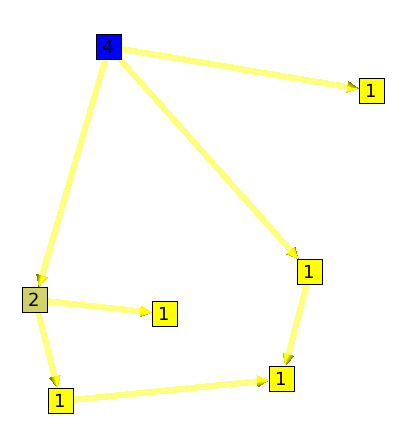
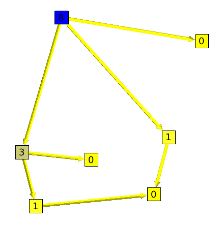
The leaf algorithm will compute for each node its number of leaves.
Here is an example :
Algorithm documentation
Here is an example :
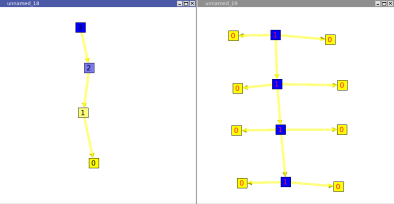
A segment, is a set of nodes that are all on one and only path. The graph showed on the left side of the example is a segment.
The segment algorithm will count, for all nodes, its number of edges without ramification.
Following are two graphs. On the left one you can see that the root "has" 3 edges without ramification. But, on the right graph all nodes (without considering leaves) have only 1 edge without ramification.
Compute the maximum outdegree of the nodes in the subtree induced by each node. To access to the degree of a node it is recommended to use directly the degree function available in each Graph.
Algorithm documentationWarning ! : Some of the following algorithm have no effect if the option "Force Ratio" is checked.
This algorithm can only be applied to 3-connected graphs. A graph G is said to be 3-connected if there does not exist a set of 2 nodes whose removal disconnects the graph. (Triangle Layout)
Algorithm documentation- The edges should not cross each other.
- The polyline used to draw an edge should have the least possible bends.
- The minimal angle between two adjacent edges of a node n should be nearest to 2pi / deg (n). This property will improve the angular resolution.
- The order of children of a node should be respected in the final drawing.
Here is an example :
The following graph has the default layout (hierarchical layout). It has a pretty bad angular resolution. Indeed, we do not see the leaves, but only a large black rectangle of edges.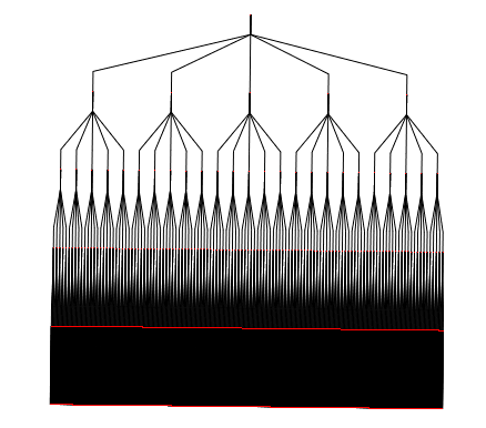
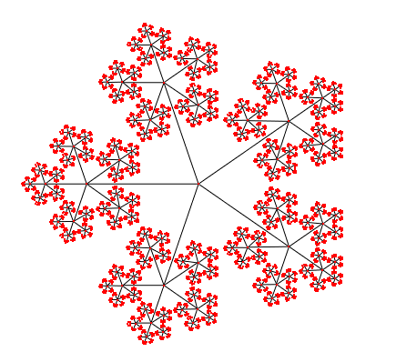
- node size : size of the node will depend of the metric that you choose. The Algorithm will consider that parameter so that no nodes overlap themselves. This can be useful, if you want a node to be far from the others, just take a new size Metric and give a higher value to that specific node.
- Orientation : Vertical / Horizontal
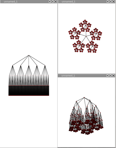
The dendrogram layout is a hierarchical layout on which every leaves are displayed on the same layer.
A dendrogram is a tree diagram frequently used to illustrate the arrangement of the clusters produced by a clustering algorithm. Dendrograms are often used in computational biology to illustrate the clustering of genes.
The algorithm takes 4 parameters :
- node size : size of the node will depend of the metric that you choose. The Algorithm will consider that parameter so that no nodes overlap themselves. This can be useful, if you want a node to be far from the others, just take a new size Metric and give a higher value to that specific node.
- orientation : up to down, left to right, right to left or down to up.
- layer spacing : space between the levels of the Tree.
- node spacing : space between sibling nodes.
- node size : size of the node will depend of the metric that you choose. The Algorithm will consider this parameter so that no nodes overlap themselves. This can be useful, if you want a node to be far from the others, just take a new size Metric and give a higher value to that specific node.
- edge length : this parameter can take a property of type int, and will be used to place a node on a specific layer. If its value is 1, no thing will happen, but if its value is 2, the node will be placed on the next layer.
- orientation : vertical/horizontal;
- orthogonal : enables the drawing of the edges, orthogonally bent.
- layer spacing : space between the levels of the Tree.
- node spacing : space between nodes sibling nodes.
- bounding circle : if checked, the estimation of overlapping nodes will be computed with bounding circles instead of bounding rectangles.
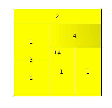
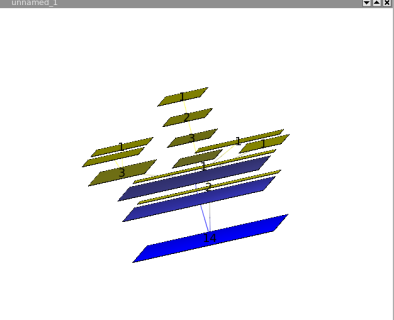
The squarified tree map layout, will place nodes in nested rectangles. For example, lets take a tree with a root and two sons, the layout will draw a rectangle for the root containing two other rectangles (its sons). This layout can be very useful for analyzing disks usages.
Here is an example :
Following is the tree a a file system containing 6 file of 1Mb, and severals directories.
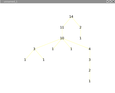
This layout looks like the improved walker, but does not pack the nodes. The result is a nice hierarchical tree in which nodes does not overlap.
Algorithm documentationOn this layout, nodes of the same layer are placed on a circle whose center is the root.
Algorithm documentation- node size : size of the node will depend of the metric that you choose. The Algorithm will consider that parameter so that no nodes overlap themselves. This can be useful, if you want a node to be far from the others, just take a new size Metric and give a higher value to that specific node.
- Rotation.
- Coordinates.
- Complexity.
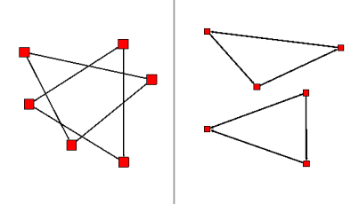
Here is an example (left = before, right = after)
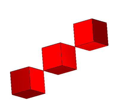
This layout can be used to see a correlation between 3 metrics (parameters). For example, if we have a node with "usedMetric1" = 0, "usedMetric2" = 1 and, "usedMetric3" = 2, the node will be place in the space with the coordinates : (0,1,2).
Following is an example, in which are 3 nodes. Those 3 nodes have 3 Metrics (called x,y,z). Node 1 equals to (0,0,0), Node 2 equals to (1,1,1) and Node 3 equals to (2,2,2).
We can see from the layout, that our correlation follow a linear function.
Force Directed layouts will try to place nodes so that, the distance in the graph (metric of the edges) should be the closest to the distance on the drawing.
Warning ! : The previous property is not true at 100%.
The GEM layout, unlike the HDE layout, works on all graphs. But it can take a very long computing time if the graph has more than 2000 nodes.
Algorithm documentationThis layout, will place the nodes of a graph as if the graph was a tree.
Algorithm documentationThis layout is the same that the "Hierarchical Graph" but in 3D.
Algorithm documentationConvolution clustering is an approach to partitioning a graph that gives the user interactive control over how many clusters to create. Tulip calculates a density function based on the chosen metric, displays a convolution of its histogram, and partitions the graph according to the humps in the histogram.
This algorithm will create sub-graphs in which all nodes or all edges (not both a the same time), have the same value.
This algorithm will divide the graph in 2 different subgraphs; the first one will contain nodes that have the viewMetric value under than a certain limit, and, the other one, in which nodes will have a the viewMetric value higher than the limit. Then, the algorithm will be re-applied to the subgraph (the one with higher viewMetrics) until the subgraph contains less than 10 nodes.
Algorithm documentationParameters :
oriented :This parameter indicates whether the graph has to be considered as oriented or not.
node function :This parameter enables to choose the function used to compute a measure value for a meta-node using the values of its underlying nodes.
edge function :This parameter enables to choose the function used to compute a measure value for a meta-edge using the values of its underlying edges.
edge cardinality :This parameter indicates whether the cardinality of the underlying edges of the meta-edges has to be computed or not. If yes, the property edgeCardinality will be created for the quotient graph.